
Baccalauréat
Physique
D & TI
2013
Correction
Bonjour ! Groupe telegram de camerecole, soumettrez-y toutes vos préoccupations. forum telegram
Exercice 1: Mouvements dans les champs de forces
1.1. Champ de pesanteur
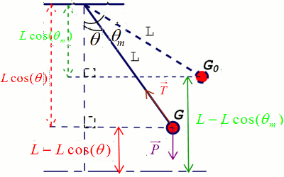
1.1.1 Vitesse du pendule au point G. en utilisant le théorème de l’énergie cinétique, nous avons:
\({E_{{C_G}}} - {E_{{C_0}}}\) \( = W(\overrightarrow P ) + W(\overrightarrow T )\)
\(\frac{1}{2}mv_G^2 - \frac{1}{2}mv_0^2\) \( = - mg({z_G} - {z_{{G_0}}})\) \( = - mg((l - l\cos (\theta ))\) \( - (l - l\cos ({\theta _0})))\) \( = mgl(\cos (\theta ) - \cos ({\theta _0}))\)
\(v_G^2 - v_0^2\) \( = 2gl(\cos (\theta ) - \cos ({\theta _0}))\) \({v_G}\) \( = \sqrt {v_0^2 + 2gl(\cos (\theta ) - \cos ({\theta _0}))} \)
\({\color{blue}{v_G} = 10,23{\rm{m/s}}}\)
1.1.2.a) schéma
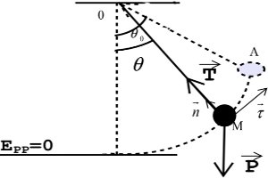 1.1.2.b. Exprimons l’intensité T de la torsion du fil en fonction de v, L, θ, θ 0 ,m et g
Il est soumis à l’action du poids et à la tension du fil.
Supposons le référentiel d’étude galiléen et appliquons le TCI dans la base de Frenet
\(\overrightarrow P + \overrightarrow T \) \(m\overrightarrow {{a_G}} \Rightarrow \) \(\overrightarrow P {\left( \begin{array}{l} - mg\cos (\theta )\\ - mg\sin (\theta )\end{array} \right)_{\overrightarrow {n,} \overrightarrow \tau }}\) \( + \overrightarrow T {\left( \begin{array}{l}T\\0\end{array} \right)_{_{\overrightarrow {n,} \overrightarrow \tau }}}\) \( = m{\overrightarrow a _G}{\left( \begin{array}{l}\frac{{{v^2}}}{l}\\l\ddot \theta \end{array} \right)_{_{\overrightarrow {n,} \overrightarrow \tau }}}\)
Suivant le vecteur \({\overrightarrow \tau }\) nous avons
\( - mg\cos (\theta ) + T\) \( = m\frac{{{v^2}}}{l}\)
\( \Rightarrow T\) \( = m\frac{{{v^2}}}{l} + mg\cos (\theta ){\rm{ }}\) avec \({v^2} = \) \(v_0^2 + 2gl(\cos (\theta ) - \cos ({\theta _0}))\)
\(T = \) \(m\frac{{v_0^2}}{l}\) \( + mg(3\cos (\theta )\) \( - 2\cos ({\theta _0}))\) \(T = 10,923{\rm{N}}\)
1.2. Champ électrostatique
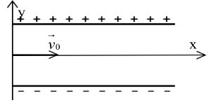
a) Faisons le schéma montrant le condensateur, la vitesse initiale et les axes du repère choisi.
 b) L’équation cartésienne de la trajectoire du positron est la suivante
\(y = \frac{{e.E}}{{2mv_0^2}}{x^2}.\)
Le positron étant de chaque positive +e
c) Donnons l’allure des deux trajectoires
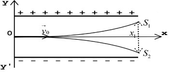
d) Calculons la distance d = S1S2.
\({S_1}\left( \begin{array}{l}{x_1}\\{y_1}\end{array} \right){\rm{ }}\) et \({S_2}\left( \begin{array}{l}{x_1}\\{y_2}\end{array} \right)\) \( \Rightarrow {S_1}{S_2}\) \( = \sqrt {{{({x_1} - {x_1})}^2} + {{({y_1} - {y_2})}^2}} \) \( = \sqrt {{{({y_1} - {y_2})}^2}} \) \( = \left| {{y_1} - {y_2}} \right|\)
Avec: \({y_1} = - \frac{{e.E}}{{2mv_0^2}}{l^2}{\rm{ }}\) et \({\rm{ }}{y_2} = \frac{{e.E}}{{2mv_0^2}}{l^2}\)
\({S_1}{S_2} = d = \frac{{e.}}{{mv_0^2}}{l^2}\frac{U}{L}\) \({S_1}{S_2} = d = 4,44 \times {10^{ - 2}}{\rm{m}}\)
Exercice 2: Système mécanique oscillant
2.1 Il est soumis à l’action du poids et à la tension du fil.
Supposons le référentiel d’étude galiléen et appliquons le TCI dans la base de Frenet
Il est soumis à l’action du poids et à la tension du fil.Supposons le référentiel d’étude galiléen et appliquons le TCI dans la base de Frenet
\(\overrightarrow P + \overrightarrow T \) \( = m\overrightarrow {{a_G}} \Rightarrow \) \(\overrightarrow P {\left( \begin{array}{l} - mg\cos (\theta )\\ - mg\sin (\theta )\end{array} \right)_{\overrightarrow {n,} \overrightarrow \tau }}\) \( + \overrightarrow T {\left( \begin{array}{l}T\\0\end{array} \right)_{_{\overrightarrow {n,} \overrightarrow \tau }}}\) \( = m{\overrightarrow a _G}{\left( \begin{array}{l}\frac{{{v^2}}}{l}\\l\ddot \theta \end{array} \right)_{_{\overrightarrow {n,} \overrightarrow \tau }}}\)
Suivant le vecteur \({\overrightarrow \tau }\) nous avons
\( - mg\sin (\theta )\) \( + 0 = ml\ddot \theta \) et \({\theta _0} \prec {10^0}\) avec \(\sin (\theta ) \approx \theta \)
L’équation différentielle devient donc
\(\ddot \theta + \frac{g}{l}\theta = 0\)
2.2. Calcule la longueur l de ce pendule.
\(\omega _0^2 = \frac{g}{l}\) \( = 4{\pi ^2}f_0^2\) \( \Rightarrow l = \frac{g}{{4{\pi ^2}f_0^2}}\) \(l = 0,57{\rm{m}}\)
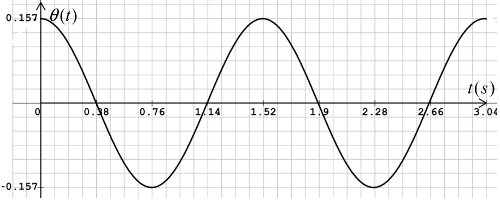
2.3 L’équation horaire θ = g(t) du mouvement
L’oscillateur étant harmonique, son équation horaire est de la forme
\(\theta (t) = {\theta _0}\sin ({\omega _0}t + \varphi )\)
À t=0, θ(0) =θ0 =90 \(\left. \begin{array}{c}{360^0} \to 2\pi {\rm{ rad}}\\{{\rm{9}}^{\rm{0}}} \to x\end{array} \right\}\) \( \Rightarrow x = \frac{\pi }{{20}}{\rm{ rad}}\)
\(t = 0s,{\rm{ }}\) \(\theta (0) = {\theta _0}\) \( = {\theta _0}\sin (\varphi )\) \( \Rightarrow \sin (\varphi )\) \( = 1\left\{ \begin{array}{l}\varphi = \frac{\pi }{2}\\\varphi = \frac{{3\pi }}{2}\end{array} \right.\)
La vitesse étant positive à l’instant initiale, nous avons \(\varphi = \frac{\pi }{2}\) rad
\(\theta (t)\) \( = \frac{\pi }{{20}}\sin ({\omega _0}t + \frac{\pi }{2})\)
2.4. Traçons la courbe θ = g(t)
Exercice 3: Radioactivité et propagation des ondes
3.1. Radioactivité:
3.1.1 a) Ecrivons l’équation générale de la réaction globale.
\({}_{92}^{238}U \to \) \({}_{82}^{206}Pb + x{}_2^4He + y{}_{ - 1}^0e\)
3.1.1.b ) calcule x et y.
D’après la loi de Soddy, nous avons
\(\left\{ \begin{array}{l}238 = 206 + 4x\\92 = 82 + 2x - y\end{array} \right.\) \( \Rightarrow x = 8{\rm{ et }}y = 6\)
3.2.1 Déterminons le temps t qu’il faudra pour qu’elle soit divisée par 1500.
\(A(t) = {A_0}\exp ( - \lambda t)\) avec \(A(t) = \frac{{{A_0}}}{{1500}}\)
\(\frac{{{A_0}}}{{1500}}\) \( = {A_0}\exp ( - \lambda .t)\) \( \Rightarrow t = \frac{1}{\lambda }\ln 1500\) \( = \frac{T}{{\ln 2}}\ln 1500\)
\(\color{blue}{t = 73,85\min }\)
3.2. Propagation des ondes mécaniques
3.2.1. Calcule la célérité V des ondes.
\({\rm{V}} = \lambda .f = 0,308{\rm{m/s}}\)
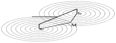
3.2.2 Dessinons l’aspect de la surface libre de l’eau comprise entre les deux extrémités de la fourche.
3.2.3 Les franges d’interférences se resserrent car, de la formule v=λf , si v reste constante, λ doit diminuer.
Exercice 4 Exploitation d’une fiche de T.P
5.1. Tracer la courbe x = f(t2)
| \({T^2}({s^2})\) | 0 | 4 | 14 | 36 | 42,25 |
| x (m) | 0 | 0,19 | 0,77 | 1,73 | 2,03 |
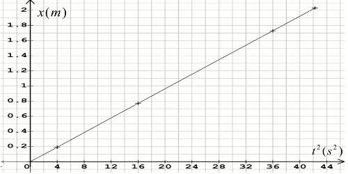 5.2 La courbe est une droite donc l’équation est de la forme: \(x(t) = a.{t^2}\)
5.3 justification
•Un fil étant inextensible de masse négligeable, la poulie étant également de masse négligeable
\({a_B} = {a_A}\) \( = r\ddot \theta = {a_G}\)
5.4 Montrons que l’accélération a commune de M et de M’ est de la forme: \({a_G} = \frac{m}{{2M + m}}g\)
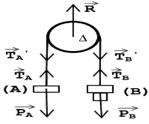
En effet: d’après le schéma nous avons, à partir du TCI:
Pour le solide (A)
\({\overrightarrow P _A} + {\overrightarrow T _A}\) \( = {m_A}{\overrightarrow a _G}\) \( \Leftrightarrow {\overrightarrow P _A}\left| \begin{array}{l}0\\ - {P_A}\end{array} \right.\) \( + {\overrightarrow T _A}\left| \begin{array}{l}0\\{T_A}\end{array} \right.\) \( = {m_A}{\overrightarrow a _G}\left| \begin{array}{l}0\\{a_G}\end{array} \right.\)
Soit : \( \color{blue}{- {P_A} + {T_A}}'\) \( \color{blue}{= {m_A}{a_G}}{\rm{ \color{red}{\ (1)}}}\)
Pour le solide (B)
\({\overrightarrow P _B} + {\overrightarrow T _B}\) \( = {m_B}{\overrightarrow a _G}\) \( \Leftrightarrow {\overrightarrow P _B}\left| \begin{array}{l}0\\{P_B}\end{array} \right.\) \( + {\overrightarrow T _B}\left| \begin{array}{l}0\\ - {T_B}\end{array} \right.\) \( = {m_B}{\overrightarrow a _G}\left| \begin{array}{l}0\\{a_G}\end{array} \right.\)
Soit : \({\color{blue}{P_B} - {T_B}}\) \(\color{blue}{ = {m_B}{a_G}}{\rm{\color{red}{\ (2)}}}\)
D’après le principe des actions réciproques
\({T_A} = {T_A}'\) et \({T_B} = {T_B}'\)
La masse de la poulie étant négligeable, nous avons:
\({\mathfrak{M}_\Delta }({T_A}')\) \( + {\mathfrak{M}_\Delta }({T_B}')\) \( = {J_\Delta }\ddot \theta = 0\)
\( - r{T_A}' + r{T_B}'\) \( = 0 \Rightarrow \)\({T_A}' = {T_B}'\)
Ainsi : \({T_A} = {T_B}\) \( = {m_B}.g - {m_B}{a_G}\) \( = {m_A}.g + {m_A}{a_G}\)
\({a_G} = \frac{{{m_B} - {m_A}}}{{{m_B} + {m_A}}}g\) \( = \frac{{M + m - M}}{{M + m + M}}g\) \( = \frac{m}{{m + 2M}}g\)
La loi horaire des ( A ) et ( B ) système est dont de la forme
\(x(t)\) \( = \frac{1}{2}.\frac{m}{{(m + 2M)}}g.{t^2}\)
- Déterminons la valeur expérimentale gexp de l’accélération de la pesanteur du lieu de l’expérience
De la droite précédente, nous avons la pente suivante:
\(p = \tan (\theta )\) \( = \frac{{\Delta x}}{{\Delta {t^2}}}\) \( = \frac{{2,03 - 0,2}}{{42,25 - 4}}\) \( = 47,85 \times {10^{ - 3}}\) \(g = \frac{{2p(m + 2M)}}{m}\) \(g = 9,667{\rm{N/kg}}\)
