Une fonction réelle d'une variable réelle associe une valeur réelle à tout nombre de son domaine de définition. Ce type de fonction numérique permet notamment de modéliser une relation entre deux grandeurs physiques
I- Généralité sur les fonctions
1) Définition d’une fonction
On appelle fonction toute relation de A vers B qui à chaque élément de A, on associe au plus un élément de B.
Exemple : \(f(x) = \) \({x^2} + 2\)
2) Ensemble de définition ou domaine de définition d’une fonction numérique
On appelle ensemble de définition ou domaine de définition d’une fonction numérique, l’ensemble des éléments qui ont une image par \(f\). On le note \(Df\).
Exemple : \(f(x) = \) \(\frac{{2x - 3}}{{{x^2} - 1}}\), ainsi \(f(x)\) existe si et seulement si : \({{x^2} - 1 \ne 0}\) soit \(Df = \) \( \mathbb{R}\) \(\backslash \left\{ { - 1;1} \right\}\)
II. Définition de la limite d’une fonction
II.1 Limite, limite à gauche et limite à droite
Soit \(f\) une fonction numérique d’une variable réelle et \(a\) un nombre réel.
• Si pour des valeurs de \(x\) proches de \(a\), \(f(x)\) prend des valeurs proches d’un nombre réel \(l\), on dit que \(l\) est la limite de \(f\) en \(a\).
On note \(\mathop {\lim }\limits_{x \to a} f(x) = l\).
• Si pour des valeurs de x proches de \(a\) et inférieures à \(a\), \(f(x)\) prend des valeurs proches d’un nombre réel \(l\), on dit que \(l\) est la limite de \(f\) à gauche de \(a\).
On note \(\mathop {\lim }\limits_{x \to {a^ - }} f(x) = l\)
• Si pour des valeurs de x proches de \(a\) et supérieures à \(a\), \(f(x)\) prend des valeurs proches d’un nombre réel \(l\), on dit que \(l\) est la limite de \(f\) à droite de \(a\).
On note \(\mathop {\lim }\limits_{x \to {a^ + }} f(x) = l\)
\(\mathop {\lim }\limits_{x \to a} f(x) = l\) \( \Leftrightarrow \mathop {\lim }\limits_{x \to {a^ - }} f(x)\) \( = \mathop {\lim }\limits_{x \to {a^ + }} f(x) = l\)
II.2 Opérations sur les limites
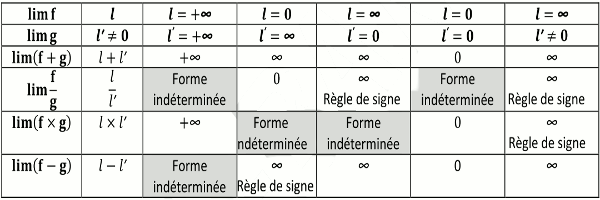
N.B : On remarque ainsi que l’on a quatre (4) formes indéterminées qui sont :
• \( - \infty + \infty \)
• \(\frac{0}{0}\)
• \(\frac{\infty }{\infty }\)
• \(0 \times \infty \)
III. Limites des fonctions élémentaires :
• Limites à l’infini d’une fonction polynôme
Soit la Fonction polynome suivante : \(f(x) = \) \({a_n}{x^n} + {a_{n - 1}}{x^{n - 1}}\) \( + ... + {a_0}\)
\(\mathop {\lim }\limits_{x \to \pm \infty } f(x) = \) \(\mathop {\lim }\limits_{x \to \pm \infty } {x^n}({a_n} + \) \(\frac{{{a_{n - 1}}}}{x} + ... + \frac{{{a_0}}}{{{x^n}}})\)
Or \(\mathop {\lim }\limits_{x \to \pm \infty } ({a_n} + \frac{{{a_{n - 1}}}}{x}\) \( + ... + \frac{{{a_0}}}{{{x^n}}}) \to {a_n}\)
\(\mathop {\lim }\limits_{x \to \pm \infty } f(x) = \) \(\mathop {\lim }\limits_{x \to \pm \infty } {x^n}{a_n}\)
• Limites à l’infini du rapport de deux fonctions polynômes
Soient \(f(x) = {a_n}{x^n}\) \( + {a_{n - 1}}{x^{n - 1}} + ...\) \( + {a_0}\) et \(g(x) = {b_n}{x^n}\) \( + {b_{m - 1}}{x^{m - 1}} + ...\) \( + {b_0}\)
\(\mathop {\lim }\limits_{x \to \pm \infty } \frac{{f(x)}}{{g(x)}} = \) \(\mathop {\lim }\limits_{x \to \pm \infty } \frac{{{a_n}{x^n} + ... + {a_0}}}{{{b_m}{x^m} + ... + {b_0}}}\) \( = \mathop {\lim }\limits_{x \to \pm \infty } \frac{{{a_n}{x^n}}}{{{b_m}{x^m}}}\)
• Limite d’une fonction composée
Soient \(f\), \(g\) et \(h\) trois fonctions telles que \(f(x) = g \circ h(x)\).
Si \(\mathop {\lim }\limits_{x \to a} h(x) = b\) et \(\mathop {\lim }\limits_{x \to b} g(x) = c\) alors \(\mathop {\lim }\limits_{x \to a} g \circ h(x) = c\)
• Limite des fonctions circulaires
Si \(a\) est un nombre réel non nul, on a :
\(\mathop {\lim }\limits_{x \to 0} \frac{{\sin x}}{x} = 1\)
\(\mathop {\lim }\limits_{x \to 0} \frac{{\sin ax}}{{ax}} = 1\)
\(\mathop {\lim }\limits_{x \to 0} \frac{{\tan x}}{x} = 1\)
\(\mathop {\lim }\limits_{x \to 0} \frac{{\tan ax}}{{ax}} = 1\)
\(\mathop {\lim }\limits_{x \to 0} \frac{{1 - \cos x}}{{{x^2}}} = \frac{1}{2}\)
\(\mathop {\lim }\limits_{x \to 0} \frac{{1 - \cos ax}}{{{{\left( {ax} \right)}^2}}} = \frac{1}{2}\)
IV Quelques théorèmes sur les limites
IV.1 Théorème de comparaison
Soient \(f\) et \(g\) sont deux fonctions admettant de limites en \(a\) où \(a\) est un élément de \( \mathbb{R}\) \( \cup \left\{ { - \infty ; + \infty } \right\}\)
Si \(f(x) \le g(x)\) alors \(\mathop {\lim }\limits_{x \to a} f(x) \le \) \(\mathop {\lim }\limits_{x \to a} g(x)\)
Conséquences
i) Si \(f(x) \le g(x)\) et \(\mathop {\lim }\limits_{x \to a} f(x)\) \( = + \infty \) alors \(\mathop {\lim }\limits_{x \to a} g(x)\) \( = + \infty \) ;
ii) Si \(f(x) \le g(x)\) et \(\mathop {\lim }\limits_{x \to a} f(x)\) \( = - \infty \) alors \(\mathop {\lim }\limits_{x \to a} g(x)\) \( = - \infty \) ;
Exemple : Calculer \(\mathop {\lim }\limits_{x \to + \infty } \left( {x + \sin x} \right)\).
IV 2. Théorème des gendarmes
Si \(g(x) \le f(x)\) \( \le h(x)\) et si en plus \(\mathop {\lim }\limits_{x \to a} g(x) = \) \(\mathop {\lim }\limits_{x \to a} g(x) = l\) alors \(\mathop {\lim }\limits_{x \to a} f(x) = l\) ;
IV.3 Théorème d’encadrement
Soient \(f\) et \(g\) deux fonctions définies sur \(\left] {a; + \infty } \right[\) et \(l \in \) \( \mathbb{R}\)
Si \(\left| {f(x) - l} \right| \le g(x)\) et si en plus \(\mathop {\lim }\limits_{x \to a} g(x) = 0\) alors \(\mathop {\lim }\limits_{x \to a} f(x) = l\).
Exemple : Montrer que \(\mathop {\lim }\limits_{x \to + \infty } \frac{{x + \sin x}}{x}\) \( = 1\)
IV.4 Théorème de l’Hôpital
Soient \(f\) et \(g\) deux fonctions continues et dérivables en un point \({x_0}\).
Si \(f({x_0}) = g({x_0})\) \( = 0\) et \(g'({x_0}) \ne 0\) alors \(\mathop {\lim }\limits_{x \to {x_0}} \frac{{f({x_0})}}{{g(x)}} = \) \(\frac{{f'({x_0})}}{{g'({x_0})}}\)
IV Utilisation du taux de variation pour déterminer la limite d’une fonction
En effet, \(\mathop {\lim }\limits_{x \to {x_0}} \frac{{f(x) - f({x_0})}}{{x - {x_0}}}\) \( = f'({x_0})\)
Exemple : Calculer \(\mathop {\lim }\limits_{x \to 0} \frac{{\sqrt {x + 1} - 1}}{x}\)
V Interprétation graphique de la limite d’une fonction : Notion d’asymptote
• Si \(\mathop {\lim }\limits_{x \to - \infty } f(x) = l\) ou \(\mathop {\lim }\limits_{x \to + \infty } f(x) = l\) , alors la droite d’équation \(y = l\) est asymptote horizontale à la courbe représentative de \(f(x)\).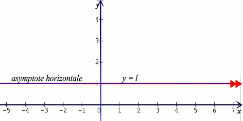
Si \(\mathop {\lim }\limits_{x \to a} f(x) = - \infty \) ou \(\mathop {\lim }\limits_{x \to a} f(x) = + \infty \) alors la droite d’équation \(x = a\) est asymptote verticale à la courbe représentative de \(f(x)\). 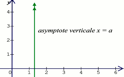
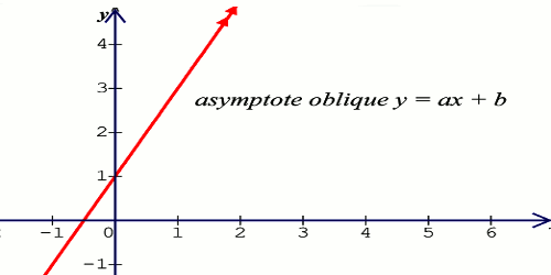
Si \(\mathop {\lim }\limits_{x \to + \infty } (f(x)\) \( - \left( {ax + b} \right) = 0\) ou \(\mathop {\lim }\limits_{x \to - \infty } (f(x)\) \( - \left( {ax + b} \right) = 0\) alors la droite d’équation \({y = ax + b}\) est asymptote oblique à la combe représentatives de \(f(x)\).